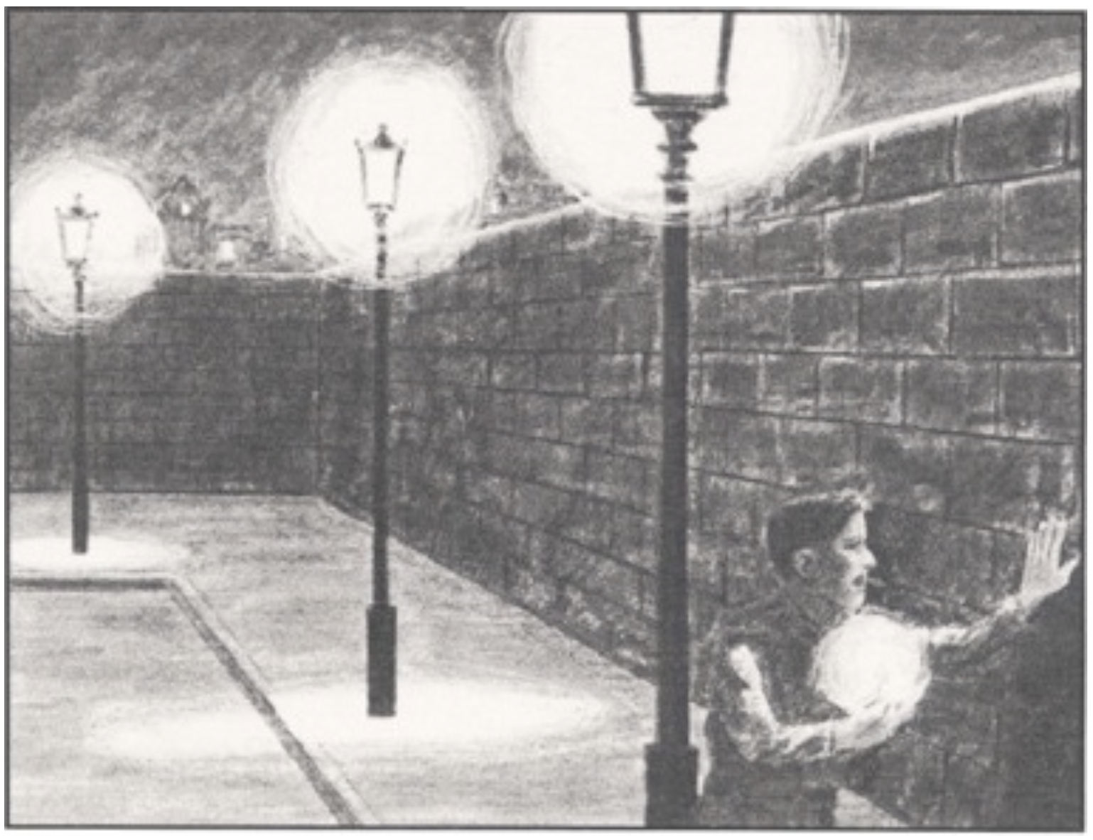
Example: The infinite wall
We are in front of a wall (infinite in both directions). We want to find the only door in it, but it is night and we can only see in front of us. How can we find the door moving left or right along the wall?
- Algorithm 1
-
go 1 meter to the right and come back, 2 to the left and come back, 3 to the right and come back, etc (at the ith step go to i meters either to the left or right and come back)
- Algorithm 2
-
go 1 meter to the right and come back, 2 to the left and come back, 4 to the right and come back, 8 to the left and come back, etc (at the ith step go to 2^i meters either to the left or right and come back)
Which algorithm makes you travel the smaller distance?
Complexity of an algorithm
computational resources it consumes: execution time, memory space, I/O, randomness, etc
Analysis of algorithms
Investigate the properties of the complexity of algorithms
- Compare alternative algorithmic solutions
- Predict the resources that an algorithm or data structure will use
- Improve existing algorithms and data structures and guide the design of novel algorithms and data structures
Given an algorithm A with input set I, its complexity or cost (in time, in memory space, in I/Os, randomness, etc.) is a function
T : I \to \mathbb N
(or \mathbb Q or \mathbb R, depending on what we want to study).
Characterizing such a function T is usually too complex and impractical due to the huge amount of information it yields. It is more useful to group the input according to their size and study T on them.
Definition 1 (Size) The size of an input x (denoted as |x|) is the number of symbols needed to code it:
- for natural number n, the binary size of n is the number of bits of the binary expansion of n. E.g. |14|_{b}=4
- for natural number n, the unary size of n is the value of n. E.g. |14|_{u}=14
- for a vector v, the size of v is the number of entries in v. E.g. |(a,\ b,\ c,\ EDA)|=4
Worst-case and Best-case complexity
Let I_n the set of inputs of size n for the algorithm A and T : I \to \mathbb N a cost function.
the best-case cost of A is the function T_{best}: \mathbb N\to \mathbb N
T_{best}(n)=\min\{T(i) \mid i\in I_n\}
(The best-case cost is not very useful…)
the worst-case cost of A is the function T_{worst}: \mathbb N\to \mathbb N
T_{worst}(n)=\max\{T(i) \mid i\in I_n\}
For every input i\in I_n, \qquad T_{best}(n)\leq T(i)\leq T_{worst}(n).
Average-case complexity
- given a probability distribution \mathcal D_n over I_n, the average-case cost of A according to \mathcal D_n is
\mathbb E_{X\sim \mathcal D_n} [T(X)]=\sum_{i\in I_n}T(i)\cdot \mathrm{Pr}_{X\sim\mathcal D_n}[X=i]\ .
For instance, the average-case cost under the uniform distribution over the set I_n is \sum_{i\in I_n}\frac{T(i)}{|I_n|}.
For every probability distribution \mathcal D_n,
T_{best}(n)\leq \mathbb E_{X\sim \mathcal D_n} [T(X)]\leq T_{worst}(n)\ .
Worst-case vs Average-case complexity
In this course we focus almost exclusively on the worst-case complexity.
Pro
- The worst-case complexity provides a guarantee on the complexity of the algorithm: the cost will never exceed the worst-case cost
- It is easier to compute than the average-case cost
Contra
- In some scenarios the worst-case complexity might give us a more pessimistic view than the average-case cost analysis
Growth rates
A fundamental feature of functions \mathbb R^+\to \mathbb R^+ is the growth rate.
Example 1
- Linear growth: f(n) = a·n+ b, that is f(2n) \approx 2f(n)
- Quadratic growth: g(n) = a·n^2 + b·n+ c, that is g(2n) \approx 4·g(n)
Linear and quadratic functions have different rates of growth. We can also say that they are of different orders of magnitude.
| \log_2 n |
N_1 |
2^{100}N_1 |
2^{1000}N_1 |
| n |
N_2 |
100N_2 |
1000N_2 |
| n^2 |
N_3 |
10N_3 |
31.6N_3 |
| n^3 |
N_4 |
4.64N_4 |
10N_4 |
| 2^n |
N_5 |
N_5 + 6.64 |
N_5 + 9.97 |
We want a notation to express growth rate of the cost of algorithms and for it to be independent of multiplicative constants.
We do not want that the cost of an algorithm to depend on implementations.
Asymptotic Notation
In computer science, we use asymptotic notations to classify algorithms according to how their run time (or space) requirements grow as the input size grow:
- Big Oh \mathcal O
- Big Omega \Omega
- Big Theta \Theta
- …
The \mathcal O, \Omega, \Theta notations do not refer directly to algorithms, but to the growth rate of functions.
Big-oh \mathcal O(\cdot) — definition
\mathcal O(f) (big-Oh of f) is the set of functions from \mathbb R^+ to \mathbb R^+ that eventually grow no faster than a constant times f. That is, a function g is in \mathcal O(f) if there exists a positive constant c such that g(x) \le cf(x) for all x from some value x_0 onwards.
Definition 2 Given a function f:\mathbb R^{+}\to\mathbb R^{+} the set \mathcal O(f) is
\mathcal O(f) = \{g: \mathbb R^{+}\to\mathbb R^{+}\,\vert\,\exists x_{0}\,
\exists c>0\,\forall
x\ge x_{0}\ \ g(x) \le c f(x)\}\ .
Example 2 3x^3+4x^2-5x+6\in \mathcal O(x^3)
Proof
We need to find constants c>0 and x_0 such that for every x\geq x_0, 3x^3+4x^2-5x+6\leq cx^3.
We have that 3x^3+4x^2-5x+6\leq (3+4+5+6)x^3=18x^3 whenever x\geq 1. Hence we can take x_0=1 and c=18 (for example).
Exercise 1 Show that a_kx^k+a_{k-1}x^{k-1}+\cdots +a_1x+a_0\in \mathcal O(x^k) whenever the a_is are constants and a_k>0.
Knuth’s Big-Omega \Omega(\cdot) — definition
Definition 3 Given a function f:\mathbb R^{+}\to\mathbb R^{+} the set \Omega(f) is
\Omega(f) = \{g: \mathbb R^+\to \mathbb R^+ \mid g\in \mathcal O(f)\}
In other words, \Omega(f) (big-Omega of f) is the set of functions that eventually grow at least as fast as a positive constant times f.
Big-Theta \Theta(\cdot) — definition
Definition 4 Given a function f:\mathbb R^{+}\to\mathbb R^{+} the set \Theta(f) is
\Theta(f) = \mathcal O(f)\cap \Omega(f)
The \Theta notation is more informative than the \mathcal O notation. For example, we will see in a couple of classes that an algorithm, the Binary Search, has cost \Theta(\log n). Therefore saying that it has cost \mathcal O(2^n) is also technically correct but not very informative.
Example
For every
k\in \mathbb N,
\displaystyle\sum_{i=1}^n i^k \in \Theta(n^{k+1}).
Proof
For every integer i\leq n it always holds that i^k\leq n^k, therefore
\sum_{i=1}^n i^k\leq \underbrace{n^k+\cdots+n^k}_n=n\cdot n^k=n^{k+1}\ .
That is \sum_{i=1}^n i^k\in \mathcal O(n^{k+1}).
To show that \sum_{i=1}^n i^k\in \Omega(n^{k+1}) notice that for every i\geq n/2, i^k\geq (\frac{n}{2})^k. Therefore,
\sum_{i=1}^n i^k=\sum_{i=1}^{n/2} i^k+\sum_{i=n/2+1}^{n} i^k\geq \sum_{i=n/2+1}^{n} i^k \geq \frac{n}{2}\left(\frac{n}{2}\right)^k=\frac{1}{2^{k+1}}n^{k+1}\ .
That is \sum_{i=1}^n i^k\in \Omega(n^{k+1}).
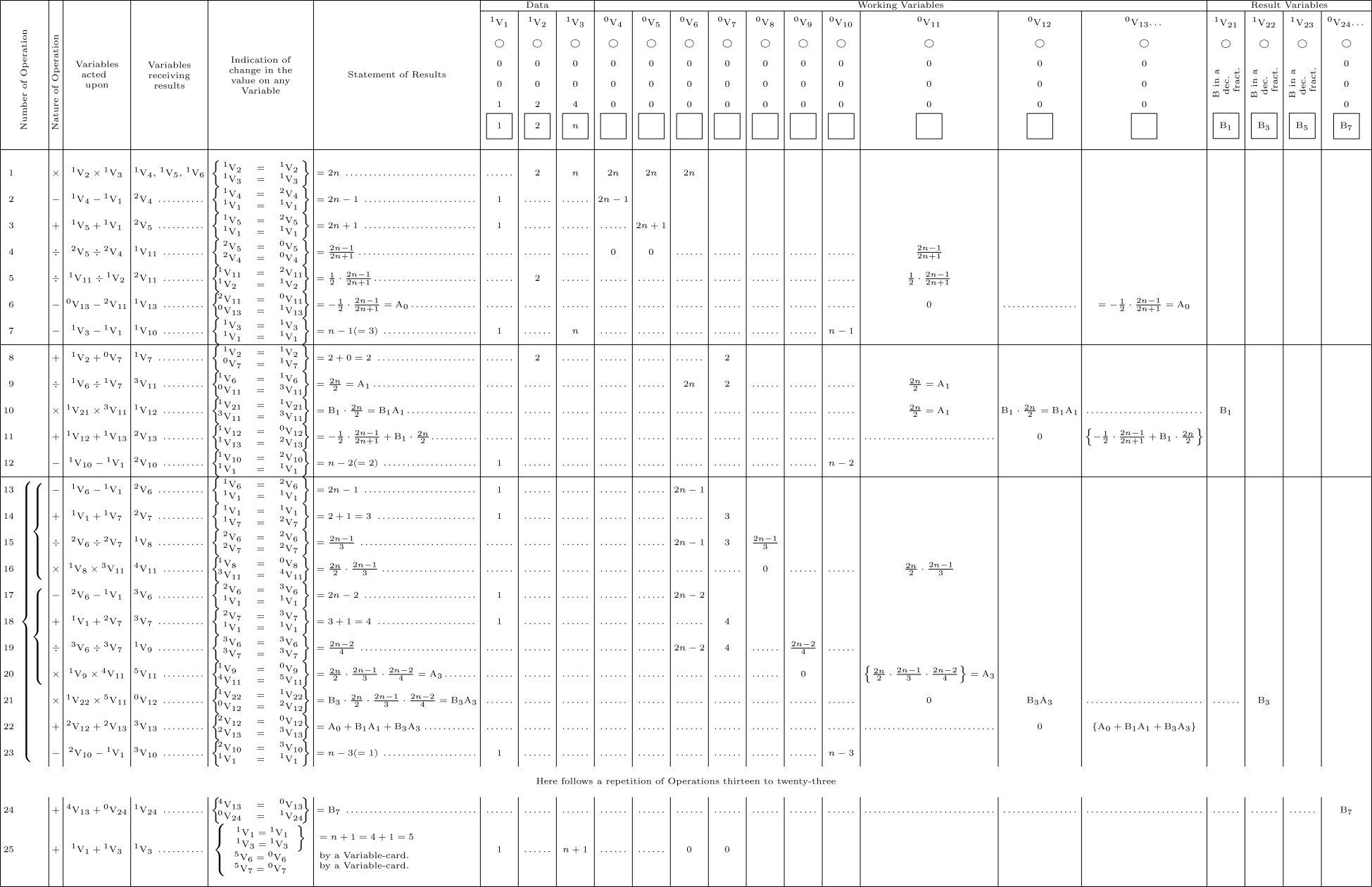
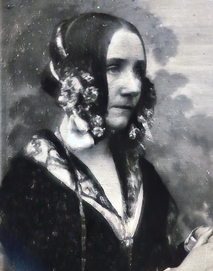
\sum_{i=0}^n i^k is actually a polynomial of degree n^{k+1} and its coefficients are related to the Bernoulli numbers. Such numbers are what Ada Lovelace in her program wanted to compute.
On notation: “=” vs “\in”
Although \mathcal O(f), \Omega(f) and \Theta(f) are set of functions, people usually use the “=” instead of the “\in”, for instance write g = \mathcal O(f) instead of g\in\mathcal O(f), or g=\Theta(f) instead of g\in \Theta(f).
This use is not symmetric: \mathcal O(f) = g, \Omega(f)=g, and \Theta(f)=g are nonsensical.
Basic properties
Assume f,g,h:\mathbb R^{+}\to\mathbb R^{+}.
- reflexivity
-
f = \mathcal O(f), f = \Omega(f), f = \Theta(f)
- transitivity
-
- if f = \mathcal O(g) and g = \mathcal O(h) then f = \mathcal O(h)
- if f = \Omega(g) and g = \Omega(h) then f = \Omega(h)
- if f = \Theta(g) and g = \Theta(h) then f = \Theta(h)
On the constants
For every positive real number c,
- \mathcal O(f) = \mathcal O(c f)
- \Omega(f) = \Omega(c f)
- \Theta(f) = \Theta(c f)
That is, we talk about \mathcal O(n) and not about \mathcal O(2n) (they are the same).
Since \mathcal O(\log_b(x))=\mathcal O(\log_c(x)), we also omit the base of logarithms and talk about \mathcal O(\log x).
Why \mathcal O(\log_b(x))=\mathcal O(\log_c(x))?
Because \log_c(f)=\frac{\log_b(x)}{\log_b(c)} and \frac{1}{\log_b(c)} is a constant.
Common error!
The constants are not always irrelevant, for instance in the exponent they are super relevant!
- \mathcal O(2^{n})\neq \mathcal O(2^{2n})
- \mathcal O(2^{\log_2(n)})\neq \mathcal O(2^{\log_3(n)})
Exercise 2 The sets \mathcal O(2^{n}) and \mathcal O(2^{2n}) are one included in the other. Which is the larger one? Same question for \mathcal O(2^{\log_2(n)}) and \mathcal O(2^{\log_3(n)}). How they relate with \mathcal O(n)?
How to decide whether f\in\mathcal O(g)?
Use the definition or, if you are lucky and \displaystyle\lim_{n\to+\infty}\frac{f(n)}{g(n)} exists, this will tell you the answer.
\small
\lim_{n\to+\infty}\frac{f(n)}{g(n)} =
\begin{cases}
0 & \Rightarrow f\in\mathcal O(g)\ (\text{and}\ f\notin \Omega(g))\\
c\qquad (0<c<+\infty)& \Rightarrow f\in\Theta(g)\\
+\infty & \Rightarrow f\in \Omega(g)\ (\text{and}\ f\notin \mathcal O(g))
\end{cases}
Computing \displaystyle\lim_{n\to+\infty}\frac{f(n)}{g(n)} does not always give an answer, for instance \sin(n)+2=\Theta(1), but clearly \displaystyle\lim_{n\to+\infty}\sin(n)+2 does not exist.
Additional properties
Assume f is an increasing function, and a,b two constants
- if a<b, \mathcal O(f^a)\subsetneq \mathcal O(f^b)
- if b>0, \mathcal O((\log f)^a)\subsetneq \mathcal O(f^b)
- if b>1, \mathcal O(f^a)\subsetneq \mathcal O(b^f)
We extend conventional operations on functions such as sums, substractions, division, powers, (etc) to classes of functions:
A\otimes B =\{h \mid \exists f\in A\ \exists g\in B\ h=f\otimes g\}\ ,
where A and B are two sets of functions and \otimes a generic operation (+, -, \cdot, /, …).
When f is a function and A a set of functions we use f \otimes A as an alias for \{f\}\otimes A.
With these conventions we can now make sense of expressions such as n+ \mathcal O(\log n), n^{\mathcal O(1)}, or \Theta(1) + \mathcal O(1/n).
Sums and Products
\mathcal O(f)+\mathcal O(g)=\mathcal O(f+g)=\mathcal O(\max\{f,g\})
(same for \Omega and \Theta)
\mathcal O(f)\cdot \mathcal O(g)=\mathcal O(f\cdot g)
(same for \Omega and \Theta)
Exercise 3 Prove the above equalities from the definition of \mathcal O.
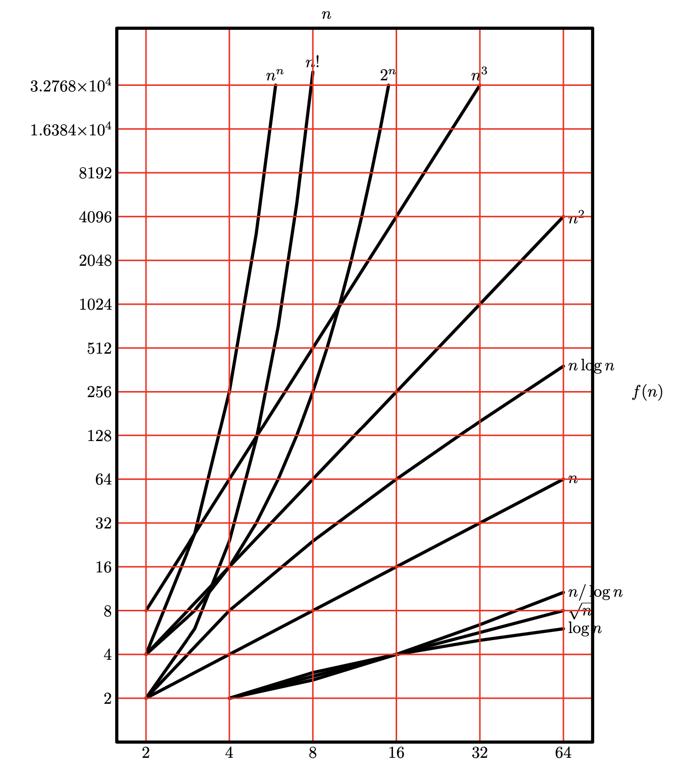
Common growth types
- Constant \Theta(1)
-
Decide whether a number is even or odd
- Logarithmic \Theta(\log n)
-
Dichotomic search on a vector of size n
- Radical \Theta(\sqrt{n})
-
Basic primality test on n
- Linear \Theta(n)
-
Linear search in an unordered vector of size n
- Quasilinear \Theta(n\log n)
-
Efficient ordering of a vector of size n
- Quadratic \Theta(n^2)
-
Sum of two n\times n matrices (with 0/1 entries)
- Cubic \Theta(n^3)
-
Product of two n\times n matrices (with 0/1 entries), using the trivial algorithm
- Polynomic \Theta(n^k)
-
Enumerate all subsets of size k in a set of size n
- Exponential \Theta(2^n)
-
Enumerate all subsets of a set of size n
- Other (n! or n^n)
-
…
Example: The infinite wall (cont’d)
We are in front of a wall (infinite in both directions). We want to find the only door in it, but it is night and we can only see in front of us. How can we find the door moving left or right along the wall?
- Algorithm 1
-
go 1 meter to the right and come back, 2 to the left and come back, 3 to the right and come back, etc (at the ith step go to i meters either to the left or right and come back)
- Algorithm 2
-
go 1 meter to the right and come back, 2 to the left and come back, 4 to the right and come back, 8 to the left and come back, etc (at the ith step go to 2^i meters either to the left or right and come back)
Which algorithm makes you travel the smaller distance?
Assume the door is at distance n (and for simplicity n=2^k)
- Algorithm 1
-
go 1 meter to the right and come back, 2 to the left and come back, 3 to the right and come back, etc
(at the ith step go to i meters either to the left or right and come back)
T_{worst}(n)= 2\sum_{i=1}^n i + n = 2\frac{n(n+1)}{2} +n=\Theta(n^2)
- Algorithm 2
-
go 1 meter to the right and come back, 2 to the left and come back, 4 to the right and come back, 8 to the left and come back, etc
(at the ith step go to 2^i meters either to the left or right and come back)
T_{worst}(n)= 2\sum_{i=0}^{k}2^i+2^k=2(2^{k+1}-1)+2^k=5n-2=\Theta(n)
Algorithm 2 is asymptotically better
Upcoming classes
- Lab: You’ll revise the C++ standard library
- Theory: We will see how to use the asymptotic notations to analyze the cost of algorithms in a systematic way