EDA T2 — Analysis of algorithms

Ilario Bonacina

ilario.bonacina+EDA@upc.edu

This presentation is an adaptation of material from Antoni Lozano and Conrado Martinez

Agenda

Last theory class

• Introduction on complexity of algorithms
  • notion of worst-, average-, best-case cost of an algorithm
• Asymptotic notation \mathcal O, \Theta, \Omega

Today

• Cost of non-recursive algorithms
• Cost of recursive algorithms
  • Recurrences and Master Theorem/method

Before we start: Questions?

Cost of non-recursive algorithms

Computing the cost (w.r.t. time) of C++ code

elementary operations

have cost \Theta(1):

• assign a basic type (int, bool, double, …)
• increase or decrease a variable of basic type
• arithmetic operations
• read/write a basic type
• comparisons
• access to the component of a vector

evaluating an expression

the cost is the sum of the costs of the operations in the expression (included functions, if they are present)

return E

this is the cost of evaluating E + the cost of copying (assigning) the result

parameters

passing by reference has cost \Theta(1)

vectors with n entries

construct/copy/assign/pass by value/return all have cost \Theta(n)

sequential composition

code_1;
code_2;
...
code_k;

If code_i has cost c_i, the total cost is c_1+c_2+\cdots+c_k

if … else …

if (condition){
code_1;
}
else{
code_2;
}

If condition has cost d and code_i has cost c_i the cost of the code above is d+c_1 (if condition evaluates to true), otherwise d+c_2. In every case the cost is \leq d +\max\{c_1,c_2\}.

while …

while(condition){
code;
};

If the cost of code at the ith iteration is c_i and the cost of condition is d_i, and the total number of iterations is m, then the total cost of the while is \sum_{i=1}^m(c_i+d_i)+d_{m+1}\ .

(The for loops are analogous)

Example (finding the minimum in a vector)

// example of use:
// vector<int> my_vector = read_data();
// cout << "min = " << minimum(v) << endl;

template <class Elem>

Elem minimum(const vector<Elem>& v) {
    int n = v.size();
    if (n == 0) throw NullSequenceError;
    Elem min = v[0];
    for (int i = 1; i < n; ++i)
        if (v[i] < min) min = v[i];
    return min;
}

0

We assume that comparison between two Elems or assigning an Elem to a variable are elementary operations

1

The total cost is dominated by the cost of the for loop (why?). So to know the total cost we just need to compute the cost of the for loop.

2

The body of the for loop has cost \Theta(1).

3

Checking i<n is \Theta(1), incrementing i with ++i is \Theta(1), and the body of the for loop is also \Theta(1).

Hence, the cost of the for loop is m\Theta(1)=\Theta(m), where m is the number of times the loop is executed.

If the size of the input vector is n, then m=n-1 and the cost of the for loop is \Theta(n).

(To see comments on the code, hoover on the numbers in it.)

Example (Naïve matrix multiplication¹)

// Naïve Matrix Multiplication
typedef vector<double> Row;
typedef vector<Row> Matrix;
// we define a multiplication operator that
// can be used like this: Matrix C = A * B;
// Pre: A[0].size() == B.size()
Matrix operator*(const Matrix& A, const Matrix& B) {
    if (A[0].size() != B.size()) 
        throw IncompatibleMatrixProduct;
    int m = A.size();
    int n = A[0].size();
    int p = B[0].size();
    Matrix C(m, Row(p, 0.0)); 
    // C = m x p matrix initialized to 0.0
    for (int i = 0; i < m; ++i)
        for (int j = 0; j < p; ++j)
            for (int k = 0; k < n; ++k)
                C[i][j] += A[i][k] * B[k][j];
    return C;
}

1

The body of the innermost for loop has cost \Theta(1).

2

This for loop has cost \Theta(n) (using the rule of products).

3

This for loop has cost \Theta(np) (again using the rule of products).

4

This for loop has cost \Theta(npm) (again using the rule of products).

5

The cost is dominated by the cost of the most external for loop.

Indeed the other parts of the algorithm have cost \Theta(mp).

Therefore, the total cost of the algorithm is \Theta(npm).

The algorithm on the left computes the matrix C=(C_{ij})_{m\times p} product of A=(A_{ij})_{m\times n} and B=(B_{ij})_{n\times p} using the definition:

\displaystyle C_{ij} = \sum_{k=0}^{n}A_{ik}B_{kj}\ .

For square matrices, where n=m=p, the cost is \Theta(n^3).

1. This is not the most efficient algorithm for matrix multiplication! (e.g. Strassen’s algorithm \to next class)

Example (Insertion sort¹)

// Insertion-sort
template <class T, class Comp = std::less<T>>

void insertion_sort(vector<T>& A, Comp smaller) {
    int n = A.size();
    for (int i = 1; i < n; ++i) {
        // put A[i] into its place in A[0..i-1]
        T x = A[i]; 
        int j = i - 1;
        while (j >= 0 and smaller(x, A[j])) {
            A[j+1] = A[j];
            --j;
        };
        A[j+1] = x;
    }
}

0

Assume that the cost of the comparison Comp is \Theta(1) and the assignment between elements of class T also is \Theta(1).

1

The while can take any number of iterations. From 0 (when A is already sorted) to i (when A is sorted but in the reverse order).

Under the assumptions in (0), in the worst-case the cost of the while is \Theta(i), while the best-case cost is \Theta(1).

If we assume all the n! possible initial orderings of A are equally likely then, on average, the cost of the while is \approx i/2.

2

The cost of the for loop in the worst-case is \begin{align*} \sum_{i=1}^{n-1}\Theta(i)&=\Theta(\sum_{i=1}^{n-1}i)\\ &=\Theta(n^2)\ . \end{align*} The cost of the for loop in the best-case is \begin{align*} \sum_{i=1}^{n-1}\Theta(1)&=(n-1)\Theta(1)\\ &=\Theta(n)\ . \end{align*} If we assume all the n! possible initial orderings of A are equally likely then, on average, the cost of the while is \Theta(n^2).

The running time of Insertion sort for any instance is both \Omega(n) and \mathcal O(n^2).

In particular, the best-case running time is \Theta(n) and the worst-case running time is \Theta(n^2).

If we assume all the n! possible initial orderings of A are equally likely then, on average, the cost is \Theta(n^2).

You can visualize runs of this algorithm for instance here.

1. Insertion sort is one of the so-called elementary sorting algorithms.

Example (Selection sort¹)

// Selection sort
template <class T, class Comp = std::less<T>>

int posicion_max (const vector<T>& A, int m, Comp smaller) {
    int k = 0;
    for (int i = 1; i <= m; ++i)
        if (smaller(A[k],A[i]))
            k = i;
    return k; 
}
void selection_sort (vector<T>& A, Comp smaller) {
    int n = A.size();
    for (int i = n-1; i >= 0; --i) {
        int k = posicion_max(A, i, smaller);
        swap(A[k], A[i]); 
    }
}

0

Assume that the cost of the comparison Comp is \Theta(1) and the assignment between elements of class T also is \Theta(1).

1

This is \Theta(1).

2

The for loop is executed m times, so the cost is m\Theta(1)=\Theta(m).

3

The cost of position_max is \Theta(m).

4

This line has cost \Theta(i).

5

The for loop has cost \begin{align*} \sum_{i=n-1}^0\Theta(i)&=\Theta(\sum_{i=n-1}^0i)\\ &=\Theta(n^2)\ . \end{align*}

6

The selection_sort has cost dominated by the for loop. Therefore it has cost \Theta(n^2) (always, best-case, worst-case, average-case under any distribution).

Selection has cost \Theta(n^2). Always! Best-case, worst-case, average-case under any distribution.

How efficient can any sorting algorithm be?

You can visualize runs of this algorithm for instance here.

1. Selection sort is another one of the so-called elementary sorting algorithms.

Lower bound on comparison-based sorting algorithms

A comparison-based sorting algorithm takes as input an array/vector [a_1,a_2,\dots ,a_n] of n items, and can only gain information about the items by comparing pairs of them. Each comparison is of the form \text{$a_i > a_j$?}

and returns YES or NO and counts a 1 time-step. The algorithm may also for free reorder items based on the results of comparisons made. In the end, the algorithm must output a permutation of the input in which all items are in sorted order (say increasingly).

Theorem 1 Every deterministic comparison-based sorting algorithm has cost \Omega(n\log n). (This actually holds for randomized algorithms too, but the argument is a bit more subtle.)

Proof sketch

For a deterministic algorithm, the permutation it outputs is solely a function of the series of answers it receives (any two inputs producing the same series of answers will cause the same permutation to be output). So, if an algorithm always made at most k < \log_2(n!) comparisons, then there are at most 2^k < n! different permutations it can possibly output. But the total number of possible permutations is n!. So, there is some permutation it can’t output and the algorithm will fail on any input for which that permutation is the only correct answer. The final bound follows from the inequality n!\geq (n/2)^{n/2} (or Stirling approx.)

Cost of recursive algorithms

Recurrences

Recurrence on T

an equation where the function T appears in both sides, with T(n) depending on T(k) for one or more values k<n.

Given a recurrence on T usually we want a closed formula for T(n).

C(n)= \begin{cases} 1 &n=1\\ C(n-1)+n&n\geq 2 \end{cases}

For instance, C(3)=C(2)+3=C(1)+2+3=1+2+3=6.

What about C(n)? Can we give a closed form for it?

\begin{align*} C(n)&=C(n-1)+n\\ &= C(n-2) +(n-1)+n\\ &= C(n-3) + (n-2)+ (n-1)+n\\ &\quad\vdots\\ &= C(1)+2+3+\cdots+(n-2)+(n-1)+n\\ &=\sum_{i=1}^n i\\ &=\frac{n(n+1)}{2}\ . \end{align*} In particular, C(n)=\Theta(n^2).

Connection with the cost of recursive algorithms

To find a recurrence that describes the cost of a recursive algorithm we have to find:

• the recursion parameter (usually the size of the input)

• the cost of the inductive step:

  • the number of recursive calls
  • the value of the parameters of the recursive calls
  • the total cost of the extra non-recursive work

Example (recursive linear search)

// Search for x in a vector v between position 0 and position n-1
// If it filds x returns the position
// Otherwise returns -1

int linear_search(const vector<int>& v, int n, int x) {
    if (n == 0) 
        return -1;
    else if (v[n-1] == x) 
        return n-1;
    else 
        return linear_search(v, n-1, x);
}

The recursion parameter is n (the second parameter of linear_search). At the beginning it is the size of v and it represents the part of v where we have still to search for x.

The worst-case cost of linear_search is

T(n)=T(n-1)+\Theta(1)

T(n)=\Theta(what function?)

Example (recursive linear search, cont’d)

T(n)= \begin{cases} \Theta(1) & n=0\\ T(n-1)+\Theta(1)&n\geq 0 \end{cases}

We prove that T(n)=\Theta(n).

Proof

\begin{align*} T(n)&= T(n-1)+\Theta(1)\\ &= T(n-2)+\Theta(1)+\Theta(1)\\ &= T(n-3)+\Theta(1)+\Theta(1)+\Theta(1)\\ &\quad\vdots\\ &= T(1)+ (n-1)\Theta(1)\\ &=\Theta(n)\ . \end{align*}

Example (recursive binary search)

// Search for x in an *increasingly ordered* vector v between positions i and j
// If it finds x, returns the index of the position
// Otherwise returns -1

int binary_search(const vector<int>& v,int i,int j,int x) { 
    if (i <= j) {
        int k = (i + j) / 2;
        if (x < v[k])
            return binary_search(v, i, k-1, x);
        else if (x > v[k])
            return binary_search(v, k+1, j, x);
        else
            return k;
    }
    else 
        return -1;
}

The recursion parameter is the size of the interval to explore n=i-j+1. The recurrence for the worst-case cost of the algorithm is T(n)=T(n/2)+\Theta(1)\ .

Example (recursive binary search, cont’d)

T(n)= \begin{cases} \Theta(1) & n=0\\ T(n/2)+\Theta(1)&n\geq 1 \end{cases}

We prove that T(n)=\Theta(\log n).

Proof

\begin{align*} T(n)&= T(n/2)+\Theta(1)\\ &= T(n/4)+2\Theta(1)\\ &= T(n/8)+3\Theta(1)\\ &\quad\vdots\\ &= T(n/2^{\log_2 n})+ (\log_2 n)\cdot \Theta(1)\\ &= T(1)+(\log_2 n)\cdot \Theta(1)\\ &=\Theta(\log n)\ . \end{align*}

Common recurrence types

Recurrences appear often (but not always!) in one of the two following forms: (a,b,c constants and f is a function)

subtract-and-conquer

T(n)=a·T(n−c)+ f(n)

corresponds to algorithms where the non-recursive part has cost f(n) and they make a recursive calls on inputs of size n−c, for some constant c.

divide-and-conquer

T(n)=a·T(n/b)+ f(n)

corresponds to algorithms with non-recursive cost f(n) and they make a recursive calls on inputs of size (approx.) n/b, for some constant b>1.

The can be solved systematically using the Master theorems/methods.

Master Theorem for “subtract-and-conquer” recurrences

Let T(n) satisfy the recurrence

T(n)= \begin{cases} \textcolor{blue}{g(n)} & n<\textcolor{purple}{n_0}\\ aT(n-\textcolor{red}{c})+ \textcolor{darkgreen}{f(n)} & n\geq n_0 \end{cases}

where \textcolor{purple}{n_0} is a constant, \textcolor{red}{c}\geq 1,
\textcolor{blue}{g(n)} is an arbitrary function and
\textcolor{darkgreen}{f(n)}=\Theta(n^k) for some constant k\geq 0.

Then \displaystyle \quad T(n) = \begin{cases} \Theta(n^k) &\text{if } a<1\\ \Theta(n^{k+1}) &\text{if } a=1\\ \Theta(a^{n/c}) &\text{if } a>1\ .\\ \end{cases}

The case a<1 does not appear in real cases of analysis of algorithms. The case a=1 appears in practice (and we already saw an example of it, the lineal search). Next slide shows an example for a>1.

Example (Towers of Hanoi)

The Towers of Hanoi is a puzzle in which we have n disks of decreasing diameters with a hole in their center and three poles A, B and C. The n disks initially sit in pole A and they must be transferred, one by one, to pole C, using pole B for intermediate movements. The rule is that no disk can be put on top of a disk with a larger diameter.

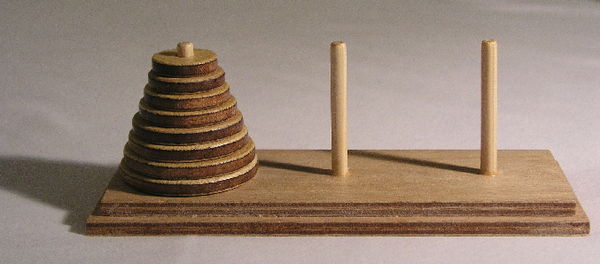
Example (Towers of Hanoi, cont’d)

typedef char pole;
// Initial call: hanoi(n,’A’, ’B’, ’C’);
void hanoi(int n, pole origin, pole aux, pole destination) {
    if (n == 1)
        cout << "Move from " << origin << " to " << destination << endl;
    else {
        hanoi(n - 1, origin, destination, aux);
        // move the largest disk
        cout << "Move from " << origin << " to " << destination << endl;
        hanoi(n - 1, aux, origin, destination);
}
}

The recurrence parameter is the number of disks to move (n). The cost of the non-recursive part is \Theta(1), and there are 2 recursive calls with recurrence parameter n-1. The recurrence describing the cost of hanoi is H(n)=2H(n-1)+\Theta(1).
By the Master Theorem (check!), H(n)=\Theta(2^n).

Master Theorem for “divide-and-conquer” recurrences

Let T(n) satisfy the recurrence

T(n)= \begin{cases} \textcolor{blue}{g(n)} & n<\textcolor{purple}{n_0}\\ \textcolor{brown}{a}T(n/\textcolor{red}{c})+ \textcolor{darkgreen}{f(n)} & n\geq n_0 \end{cases}

where \textcolor{purple}{n_0} is a constant, \textcolor{brown}{a}\geq 1 \textcolor{red}{c}> 1, \textcolor{blue}{g(n)} is an arbitrary function and \textcolor{darkgreen}{f(n)}=\Theta(n^k) for some constant k\geq 0.

Then \displaystyle \quad T(n) = \begin{cases} \Theta(n^k) &\text{if } a< c^k\\ \Theta(n^{k}\log n) &\text{if } a=c^k\\ \Theta(n^{\ln(a)/\ln(c)}) &\text{if } a>c^k\ .\\ \end{cases}

Proof sketch

Assume n=n_0c^j. \begin{align*} T(n)&=aT(n/c)+f(n)\\ &=a^2T(n/c^2)+af(n/c)+f(n)\\ &\quad \vdots\\ &=a^j T(n/c^j)+a^{j-1}f(n/c^{j-1})+\cdots+ a^2f(n/c^2)+af(n/c)+f(n)\\ &=a^j T(n_0)+a^{j-1}f(n/c^{j-1})+\cdots+ a^2f(n/c^2)+af(n/c)+f(n)\\ &= a^j g(n_0)+\sum_{i=0}^{j-1}a^if(n/c^i)\\ &=\Theta(a^j)+\sum_{i=0}^{j-1}a^i\Theta((n/c^i)^k)\\ &=\Theta(a^j)+\Theta\left(\sum_{i=0}^{j-1}a^i(n/c^i)^k\right)\\ &=\Theta(a^j)+n^k\Theta\left(\sum_{i=0}^{j-1}a^i(1/c^i)^k\right)\\ &=\Theta(a^j)+n^k\Theta\left(\sum_{i=0}^{j-1}\left(\frac{a}{c^k}\right)^i\right)\\ &=\Theta(n^{\ln(a)/\ln(c)})+n^k\Theta\left(\sum_{i=0}^{j-1}\left(\frac{a}{c^k}\right)^i\right) \end{align*} We have then 3 cases to consider according to whether \frac{a}{c^k}=1, \frac{a}{c^k}>1 or \frac{a}{c^k}<1.

• If \frac{a}{c^k}=1, then \ln(a)=k\ln(c) and \begin{align*} T(n)&=\Theta(n^{\ln(a)/\ln(c)})+n^k\Theta\left(j\right)\\ &= \Theta(n^k)+n^k\Theta(\log n)\\ &=\Theta(n^k\log n)\ . \end{align*}

If \frac{a}{c^k}\neq 1 then \sum_{i=0}^{j-1}\left(\frac{a}{c^k}\right)^i=\frac{1-(a/c^k)^{j}}{1-(a/c^k)}. We use this in the two remaining cases:

• If \frac{a}{c^k}<1, then n^{\ln(a)/\ln(c)}=\mathcal O(n^k) and \Theta\left(\sum_{i=0}^{j-1}\left(\frac{a}{c^k}\right)^i\right)=\Theta(1) and hence \begin{align*} T(n)&=\Theta(n^{\ln(a)/\ln(c)})+n^k\Theta\left(\frac{1-(a/c^k)^{j}}{1-(a/c^k)}\right)\\ &= \mathcal O(n^k)+n^k\Theta(1)\\ &=\Theta(n^k)\ . \end{align*}

• If \frac{a}{c^k}>1, then \begin{align*} T(n)&=\Theta(n^{\ln(a)/\ln(c)})+n^k\Theta\left(\frac{1-(a/c^k)^{j}}{1-(a/c^k)}\right)\\ &= \Theta(n^{\ln(a)/\ln(c)})+n^k\Theta((a/c^k)^j)\\ &=\Theta(n^{\ln(a)/\ln(c)})+\Theta(a^j)\\ &=\Theta(n^{\ln(a)/\ln(c)})\ . \end{align*} QED

The statement above still holds if instead of \frac{n}{c} in the recurrence, there is any function in \frac{n}{c}+O(1), for instance \lceil \frac{n}{c}\rceil or \lfloor \frac{n}{c}\rfloor. An example of the second case is binary search (check!).

Example (Powers)

//Exponentiation
template <typename T>

T pow(const T& a, int k) {
    if (k == 0) return identity(a);
    T b = pow(a, k/2);
    if (k % 2 == 0)
        return b*b;
    else 
        return a*b*b;
}

0

Assume the cost of identity, *, construction and copy of type T is \Theta(1).

1

Let C(k) be the cost of the algorithm.

2

C(0)=\Theta(1).

3

The if… else … part of the code has cost \Theta(1).

4

This recursive call has cost C(k/2), hence the recursion for C(k) is
C(k)=C(k/2)+\Theta(1).

This exponentiation algorithm is based on the following algebraic identity (for simplicity stated for T as int): a^k= \begin{cases} 1 & n=0\\ a^{k/2}a^{k/2} & k\text{ even}\\ a^{\lfloor k/2\rfloor}a^{\lfloor k/2\rfloor}a & k\text{ odd}\\ \end{cases}

Let C(k) be the cost of pow as a function of the exponent k. The recurrence for it is C(k)=C(k/2)+\Theta(1).

By the Master Theorem (check it!), C(k)=\Theta(\log k).

The cost of the above algorithm is actually linear in the size of the input, as k is represented with \log k bits.

Example (Fibonacci numbers)

nth Fibonacci number

F(n)=\begin{cases} 1 & n\leq 1\\ F(n-1)+F(n-2) & n\ge 2\end{cases}

// A trivial algorithm to compute 
// the n-th Fibonacci number

int fib1(int n) {
if (n <= 1) 
    return 1;
else 
    return fib1(n-1) + fib1(n-2);
}

The recurrence for the cost T(n) of fib1 is \ T(n)=T(n-1)+T(n-2)+\Theta(1).

We cannot apply the Master Theorem, but:

2T(n-2)+\Theta(1)\leq T(n)\leq 2T(n-1)+\Theta(1) Which, by the Master Theorem, gives \Omega(\sqrt{2}^n)\leq T(n)\leq \mathcal O(2^n)\ .

Actually it is possible to prove that T(n)=\Theta\left(\left(\frac{1+\sqrt{5}}{2}\right)^n\right).

Example (Fibonacci numbers, cont’d)

// A better algorithm to compute the n-th Fibonacci number

int fib2(int n) {
    if (n <= 1) return 1;
    int cur = 1;
    int pre = 1;
    for (int i = 1; i < n; ++i) {
        int tmp = pre;
        pre = cur;
        cur = cur + tmp;
    }
    return cur;
}

1

Every iteration of the for loop costs \Theta(1) and there are n iterations. Hence the total cost of the for loop is \Theta(n).

2

The total cost is dominated by the cost of the for loop and therefore it is \Theta(n).

This alternative algorithm computes the nth Fibonacci number with cost \Theta(n). Better than before, but can we do better?

Example (Fibonacci numbers, cont’d)

By induction on n (exercise), we can prove that for every n\geq 0 \begin{pmatrix} F(n+1)\\ F(n) \end{pmatrix} = \begin{pmatrix} 1&1\\ 1&0 \end{pmatrix} ^n \begin{pmatrix} 1\\ 0 \end{pmatrix}

That is we can use the rapid exponentiation algorithm pow for a couple of slides ago to compute Fibonacci numbers!

typedef vector<vector<int>> matrix;

int fib3(int n) {
    matrix f = {{1, 1}, {1, 0}};
    matrix p = pow(f, n);
    return p[1][0] + p[1][1];
}

The cost of fib3 is asyntotically the same as the cost of pow: \Theta(\log n).

Upcoming classes

• Wednesday: Problem class P1 on asymptotic notation (do the exercises before class).
• Next Monday: Theory class T3 on Divide and Conquer!

Questions?