EDA T3 — Divide and Conquer

Ilario Bonacina

ilario.bonacina+EDA@upc.edu

This presentation is an adaptation of material from Antoni Lozano and Conrado Martinez

Agenda

Last theory class

Cost of non-recursive algorithms
Cost of recursive algorithms
- Recurrences and Master Theorem/method

Today

Divide-and Conquer paradigm
- Revision of Master Theorem for divide-and-conquer recurrences
- Revision of Binary Search
- Mergesort
- Quicksort

Before we start: Questions?

Divide-and-Conquer: a template

\begin{algorithmic} \Procedure{Divide-and-Conquer}{$x$} \If{$x$ is simple} \Return{\Call{Direct-Solution}{$x$}} \Else \State $(x_1,\dots,x_k)\gets$ \Call{Divide}{$x$} \For{$i=1\ $\To $k$} \State $y_i\gets$ \Call{Divide-and-Conquer}{$x_i$} \EndFor \Return \Call{Combine}{$y_1,\dots,y_k$} \EndIf \EndProcedure \end{algorithmic}

The basic principle of divide and conquer¹ on an input x is the following:

If x is simple, find the solution using a direct method.
Otherwise, divide x into sub-instances x_1,\dots, x_k² and solve them independently and recursively.
Then combine the solutions obtained y_1,\dots, y_k to get the solution for the original input x.

Divide-and-Conquer: a template

No sub-instance of the problem is solved more than once.
The size of the sub-instances is often, at least on average, a fraction of the size of the original input, i.e., if x has size n then the average size of any x_i is n/c_i for some constants c_i > 1.¹

Divide-and-Conquer: a template

For many Divide-and-Conquer algorithms the sub-instances have (roughly) the same size and the cost T(n) satisfies a recurrence of the form:

T(n)= \begin{cases} \textcolor{blue}{g(n)} & n<\textcolor{purple}{n_0}\\ \textcolor{brown}{k}T(n/\textcolor{red}{c})+ \textcolor{darkgreen}{f(n)} & n\geq \textcolor{purple}{n_0} \end{cases}

x is “simple” if its size is \leq \textcolor{purple}{n_0}.
\textcolor{blue}{g(n)} is the cost of computing Direct-Solution(x)
\textcolor{darkgreen}{f(n)} is the cost of the Divide and Combine steps
\textcolor{brown}{k} is the number of recursive calls
\textcolor{red}{c} is the size of the sub-instances x_i

Master Theorem for “divide-and-conquer” recurrences

Let T(n) satisfy the recurrence

T(n)= \begin{cases} \textcolor{blue}{g(n)} & n<\textcolor{purple}{n_0}\\ \textcolor{brown}{a}T(n/\textcolor{red}{c})+ \textcolor{darkgreen}{f(n)} & n\geq \textcolor{purple}{n_0} \end{cases}

where \textcolor{purple}{n_0} is a constant, \textcolor{brown}{a}\geq 1 \textcolor{red}{c}> 1, \textcolor{blue}{g(n)} is an arbitrary function and \textcolor{darkgreen}{f(n)}=\Theta(n^k) for some constant k\geq 0.

Then \displaystyle \quad T(n) = \begin{cases} \Theta(n^k) &\text{if } a< c^k\\ \Theta(n^{k}\log n) &\text{if } a=c^k\\ \Theta(n^{\ln(a)/\ln(c)}) &\text{if } a>c^k\ .\\ \end{cases}

Search in a vector

Search in an ordered array

Input:

an array A[1..n] with n elements sorted in increasing order, and
some element x

Goal:

find the position i (0\leq i\leq n) such that A[i]\leq x < A[i + 1]
(with the convention that A[0] = -\infty and A[n + 1] = +\infty).

If the array were empty the answer is simple: x is not in the array.

It makes sense to work with a generalization of the original problem. (This is a typical case of parameter embedding.)

Search in an ordered subarray

Input:

a segment or subarray A[l + 1..r-1] (with 0 \leq l\leq r\leq n + 1 sorted in increasing order, and
an element x such that A[l] \leq x < A[r]

Goal:

find the position i (l\leq i<r) such that A[i]\leq x < A[i + 1].

If l + 1 = r, the segment is empty and we can return i = r- 1 = l.

Binary search

//Binary Search
// Assume A is ordered increasingly
// Initial call: int p = binary_search(A, x, -1, A.size());
template <class T>

int binary_search(const vector<T>& A, const T& x, int left, int right) {
    if (left == right + 1)
        return right;
    int mid = (left + right) / 2;
    if (x < A[mid])
        return binary_search(A, x, left, mid);
    else
        return binary_search(A, x, mid, right);
}

Link to a visualization of the algorithm

Link to another visualization

The recursion parameter is n= right - left +1

Cost of Binary search

Let n be the size of the array A where we perform the search. The cost B(n) of binary_search on an array of n elements satisfies the recurrence B(n) = \begin{cases} \text{constant} & n=0\\ B(n/2)+\Theta(1) & n>0 \end{cases} since each call makes one recursive call, either in the left or the right half of the current segment.¹ By the Master Theorem² we get B(n) = \Theta(\log n).

Applications of Binary Search

Searching in sorted arrays: Binary search is used to efficiently find an element in a sorted array.
Database queries: Binary search can be used to quickly locate records in a database table that is sorted by a specific key.
Finding the closest match: Binary search can be used to find the closest value to a target value in a sorted list.
Interpolation search: Binary search can be used as a starting point for interpolation search, which is an even faster search algorithm.

Advantages and Disadvantages of Binary Search

Pro

Efficient. Time complexity of \Theta(\log n)
Simple to implement
Versatile. Binary search can be used in a wide variety of applications.

Contra

Not suitable for unsorted data. If the array is not sorted, it must be sorted before binary search can be used.
For very large arrays (e.g., billions of elements) hash tables may be more efficient.

Code it!

Jutge exercises on variations of Binary Search

P81966 Dichotomic search
P84219 First occurrence
P33412 Resistant dichotomic search (similar to Problem 2.12 from problem class P3)
X82938 Search in a unimodal vector (similar to Problem 2.9 from problem class P3)

Sorting

Sorting: given an array sort it

Input:

an array A[1..n] with n elements

Goal:

rearrange the elements in A to have them in increasing order:
A[0]\leq A[1]\leq\cdots\leq A[n-1]

Practical uses of sorting algorithms:

online shopping
social media feeds
e-library book categorization
email management
music playlist organization
GPS navigation
digital photo management
weather forecasting
stock market analysis
medical diagnosis
scientific research
…

In the ideal world

The ideal sorting algorithm would have the following properties:

Stable: Equal entries are not reordered.
Operates in place, requiring \Theta(1) extra space.
Worst-case \Theta(n\log n) comparisons.
Worst-case \mathcal O(n) swaps.
Adaptive: Speeds up to \mathcal O(n) when data is nearly sorted or when there are few unique keys.

There is no algorithm that has all of these properties, so the choice of sorting algorithm depends on the application.

Last class:

Insertion-Sort
Selection-Sort
Every comparison-based sorting algorithm must perform at least \Omega(n\log n) comparisons to sort an n-element vector.

Today:

Mergesort
Quicksort

Mergesort

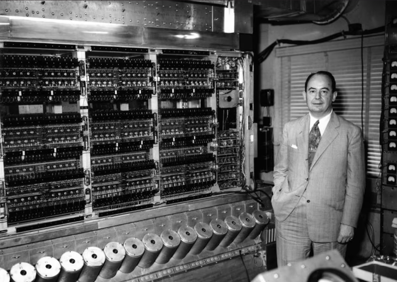
Mergesort (John von Neumann, 1945) is one of the oldest efficient sorting methods ever proposed.

Different variants of this method are particularly useful for external memory sorts. Mergesort is also one of the best sorting methods for linked lists.

The basic idea

divide the input array in two halves
sort each half recursively
get the final result merging the two sorted arrays of the previous step.

Mergesort

// Mergesort
template <typename T>

void mergesort (vector<T>& A) {
    mergesort(A, 0, A.size() - 1);
}

void mergesort (vector<T>& A, int left, int right) {
    if (left < right) {
        int mid = (left + right) / 2;
        mergesort(A, left, mid);
        mergesort(A, mid + 1, right);
        merge(A, left, mid, right);
    } 
}
// ... the code for merge is in the next slide

The heart of the algorithm is the merge part: how to merge two ordered vectors in an ordered one.

Let n= right - left +1 and T(n) be the cost of merge.

The cost M(n) of mergesort is given by the recurrence: \begin{align*} M(n)&=M\left(\lceil n/2\rceil\right) + M\left(\lfloor n/2\rceil\right) + T(n)\\ &=2M(n/2)+T(n) \end{align*}

The `merge` procedure

// The merge procedure
template <typename T>

void merge (vector<T>& A, int left, int mid, int right) {
    vector<elem> B(right - left + 1);
    int i = left; 
    int j = mid + 1; 
    int k = 0;
    while (i <= mid and j <= right) {
        if (A[i] <= A[j])
            B[k++] = A[i++];
        else 
            B[k++] = A[j++];
    }
    while (i <= mid)
        B[k++] = A[i++];
    while (j <= right)
        B[k++] = A[j++];
    for (k = 0; k <= right-left; ++k)
        A[left + k] = B[k];
}

0: Assume that assigning an element of type T, and comparisons are \Theta(1).
1: After every comparison we add an element to B.
2: If A[i]=A[j] we put in B first the element A[i]. This makes the algorithm stable (it preserves the order among equal elements of the input array).
3: We execute the while until we copy in B completely at least one of the two halves.
4: If the right part got copied completely in B we append to B the leftover of the right part.
5: Same as in (4), but with roles of the left and right part reversed.
6: We copy back in A the elements.

T(n)=\Theta(n):

The total number of comparisons between elements of type T is at most n= right - left +1.
The total number of assignments of type T is 2n

Therefore the total cost of merge is linear in n, i.e. \Theta(n)

The cost of Mergesort

The cost M(n) of mergesort is given by the recurrence: \begin{align*} M(n)&=M\left(\lceil n/2\rceil\right) + M\left(\lfloor n/2\rceil\right) + T(n)\\ &=2M(n/2)+T(n)\\ &=2M(n/2)+\Theta(n) \end{align*}

By the Master Theorem, we get that M(n)=\Theta(n\log n).

Mergesort is a stable algorithm in two senses:

it preserves the order among equal elements of the input array
its cost is always the same: it does not depend on how unordered is the input

Code it!

Jutge exercises on variations of Mergesort

P80595 How many inversions? (similar to Problem 2.11 from problem class P3)

Quicksort

Quicksort (Hoare, 1962) is a comparison-based sorting algorithm using the divide-and-conquer principle too, but contrary to the previous examples, it does not guarantee that the size of each sub-instance will be a fraction of the size of the original given instance.

The worst case cost, we will see, is \Theta(n^2), but the average cost is \Theta(n\log n) and the efficiency of its internal mechanisms make the Quicksort in practice very… quick!

Quicksort strategy vs Mergesort strategy

Mergesort

the division in sub-problems is trivial
all the non-recursive cost is in recombining the solutions
the size of the subproblems is always (roughly) half the original

Quicksort

all the non-recursive work is in partitioning into subproblems
the recombination of solutions is trivial
the size of the subproblems is not always more or less the same!

Quicksort: general template

// Quicksort
template <typename T>

void quicksort(vector<T>& A) {
    quicksort(A, 0, A.size() - 1);
}

void quicksort(vector<T>& A, int left, int right) {
    if (left < right) {
        int q = partition(A, left, right);
        quicksort(A, left, q - 1);
        quicksort(A, q + 1, right);
    } 
}

1: Here we would like to have ideally q more or less (right-left)/2 most of time during recursion. As we will see, this will not always attainable.

We examine a basic algorithm for partition, which is reasonably efficient.

Precondition of q = partition(A, left, right): 0\leq left \leq right \leq A.size()-1

Postcondition of q = partition(A, left, right): exists x s.t. for every i

left \leq i\leq q implies A[i]\leq x,
q+1 \leq i\leq right implies A[i]\geq x.

Hoare (original) partition

// Partition
// Pivot first element
#include <algorithm>
template <typename T>

int partition (vector<T>& A, int left, int right) {
    int i = left + 1;
    int j = right;
    T x = A[left];
    while (i <= j) {
        while (i <= j and A[i] <= x) ++i;
        while (i <= j and A[j] >= x) --j;
        if (i <= j) {
            swap(A[i], A[j]);
            ++i; --j;
        }
    };
    swap(A[left], A[j]);
    return j;
}
}

1: x is called pivot. We will discuss different strategies to choose it later.
2: Ideally we would like to return a value close to (left-right)/2. This depend cruacially on the choice of the value of the pivot x and how close it is to the median of A.

Let n=right-left+1.

The number of comparisons is n-1 (and the cost of partition is \Theta(n)).

Quicksort: cost analysis

To analyze the cost of quicksort we notice two facts:

it only matters the relative order of the elements to be sorted, hence we can assume that the input is a permutation of \{1,\dots,n\}.
we can focus on the number of comparisons between the elements since the total cost is proportional to that number of comparisons.

Theorem 1 (Worst-case cost of Quicksort) The worst-case cost of quicksort is \Theta(n^2).

Proof

This only occurs if in all (or most) recursive calls one of the sub-arrays contains very few elements and the other contains almost all.

For instance, this would happen if we systematically choose the first element of the current sub-array as the pivot and the array is already sorted!

In this case, we always have a very unbalanced partition: one recursive call to a sub-array of size 1 and recursive call to a sub-array of size n-1.

Since in partition the cost is always \Theta(n) this gives, for the worst-case cost T(n) of quicksort` the recurrence

T(n)=T(n-1)+\Theta(n)\ . By the Master Theorem “subtract-and-conquer” (or directly expanding the recurrence) we get T(n)=\Theta(n^2). QED

Theorem 2 (Average-case cost of Quicksort) Assume the input is a uniformly random permutation of \{1,\dots,n\} and let T(n) be the expected number of comparisons quicksort performs to sort the n elements. In particular, T(0)=0.

We have that T(n)=\Theta(n\log n).

Proof

In partition we always perform n-1 comparisons, but the size of left and right parts of the partitions might vary:

if the pivot is 1, the left part has size 0 and the right n-1,
if the pivot is 2, the left has size 1 and the right n-2, etc.

All of these n possibilities are equally likely (why?).

That is, the recurrence for T(n) is

\begin{align*} T(n)&=\sum_{j=1}^n\mathbb E[\text{\# of comparisons}\mid \text{pivot is $j$-th}]\cdot \mathrm{Pr}(\text{pivot is the $j$th}) \\ &=\sum_{j=1}^n(T(j-1)+T(n-j)+(n-1))\cdot \frac{1}{n} \\ &= (n-1)+\frac{1}{n}\sum_{j=1}^n(T(j-1)+T(n-j)) \\ &= (n-1)+\frac{2}{n}\sum_{i=1}^{n-1} T(i) \end{align*}

We prove an upper bound on T(n) by the guess-and-prove-inductively method.

We need a good guess. Intuitively, most pivots should split their array roughly in the middle, which suggests that Quicksort on average might perform similarly to Mergesort.

That is we guess that there is a constant c such that T(n)\leq cn\ln n for every n\geq 0. This is trivially true for n=0.

Assume, by induction that T(i)\leq ci\ln i for every i\leq n-1. This gives

\begin{align*} T(n)&= (n-1)+\frac{2}{n}\sum_{i=1}^{n-1} T(i) \\ &\leq (n-1)+\frac{2}{n}\sum_{i=1}^{n-1} ci\ln(i) \\ &\stackrel{(\star)}{\leq} (n-1)+\frac{2}{n}\int_{1}^n cx\ln(x)dx \\ &\stackrel{(\star\star)}{\leq} (n-1)+\frac{2c}{n}\left(\frac{1}{2}n^2\ln n-\frac{n^2}{4}+\frac{1}{4}\right) \\ &\stackrel{\text{fix }c=2}{=} (n-1)+2n\ln n-n^2+\frac{1}{n} \\ &\stackrel{(\diamond)}{\leq} 2n\ln n \end{align*}

In (\star) we used the fact that x\ln x is an increasing function, hence \sum_{i=1}^{n-1} ci\ln(i)\leq \int_{1}^n cx\ln(x)dx.
In (\star\star) we used that \int x\ln xdx=\frac{1}{2}x^2\ln x -\frac{1}{4}x^2+\text{const}.
In (\diamond) we used the fact that -n^2+n-1+\frac{1}{n}\leq 0 for every n\geq 1.

That is we proved that T(n)=\mathcal O(n\log n). Since, as we saw, for every comparison-based sorting algorithm the number of comparisons is always \Omega(n\log n), then T(n)=\Theta(n\log n). QED

Quicksort: variations on the pivot choice

Pivot: left
Pivot: random
Pivot: Median of left, center and right

// Quicksort 
// Random Pivot

template <typename T>

void quicksort(vector<T>& A, int left, int right) {
    if (left < right) {
        int q = partition(A, left, right);
        quicksort(A, left, q);
        quicksort(A, q + 1, right);
    } 
}

Pivot left

is acceptable if the input is uniformly random
if the input is ordered (increasingly or decreasingly) quicksort takes time \Theta(n^2) doing absolutly nothing useful.

// Quicksort 
// Random Pivot
#include <experimental/random>
#include <algorithm>

template <typename T>

void quicksort(vector<T>& A, int left, int right) {
    if (left < right) {
        int p = randint(left, right);
        swap(A[left], A[p]);
        int q = partition(A, left, right);
        quicksort(A, left, q);
        quicksort(A, q + 1, right);
    } 
}

Pivot random

on average divides the problem into subproblems of similar size
not always makes quicksort faster (cost of generating random numbers, etc)

// Quicksort 
// Random Pivot
#include <experimental/random>
#include <algorithm>

template <typename T>

void quicksort(vector<T>& A, int left, int right) {
    if (left < right) {
        int center = ( left + right ) / 2;
        if (A[left] < A[centre]) 
            swap(A[center], A[left]);
        if (A[right] < A[center]) 
            swap(A[center], A[right]);
        if (A[right] < A[left]) 
            swap(A[left], A[right]);
        int q = partition(A, left, right);
        quicksort(A, left, q);
        quicksort(A, q + 1, right);
    } 
}

1: After the three swaps above, we have A[\text{center}]\leq A[\text{left}] \leq A[\text{right}] So, A[\text{left}] is the median of the three.

Pivot mean of 3

the best option would be to use as pivot the median of the array of input
- too expensive to compute
the median of left, the mid element, and right is a good estimation

Quicksort: a hybrid approach

template <typename T>

void quicksort(vector<T>& A, int left, int right) {
    const int critical_size = 20;
    if ( right - left < critical_size ){
        insertion_sort(A,left,right);
    }
    else{
        int q = partition(A, left, right);
        quicksort(A, left, q);
        quicksort(A, q + 1, right);
    } 
}

For small inputs Insertion Sort is faster than Quicksort.

A good option is then to cut short the Quicksort recursion when hitting inputs of size at most a certain value (usually something between 5 and 20).

The C++ STL function stl::sort in most implementations uses a Quicksort with a hybrid approach.

More details

If the size is large enough (size \geq 16) and recursion depth is within the limit (<2 \log n), it continues sorting the data using Quicksort.
If the recursion depth is too deep, generally (>2 \log ⁡n), it switches to Heapsort as continuing with Quicksort may lead to worst case.
If the size is very small (size < 16), then it switches to Insertion sort.

Recap on sorting algorithms so far

Algorithm	Worst case	Best Case	Average case
Selection sort ¹	\Theta(n^2)	\Theta(n^2)	\Theta(n^2)
Insertion sort	\Theta(n^2)	\Theta(n) \ \ ²	\Theta(n^2)
Mergesort	\Theta(n\log n)	\Theta(n\log n) \ \ ³	\Theta(n\log n)
Quicksort	\Theta(n^2)	\Theta(n\log n) \ \ ⁴	\Theta(n\log n)

A race of sorting algorithms

Mergesort vs Quicksort speed

Upcoming classes

Wednesday: Problem class P2 on cost of algorithms (do the exercises before class).
Next Monday: Theory class T4 on more Divide and Conquer!

Questions?