Some Elementary Sorting Algorithms

We recall some basic facts on some elementary comparison-based sorting algorithms. These are sorting algorithms that only operate on the input array/vector by comparing pairs of elements and moving elements around based on the results of these comparisons.

The following tabs are about some comparison-based sorting algorithms, each contains a simple implementation of the algorithm with a reminder of the running time. You can find the implementations (and many more) also in Algorithms in C++.

Selection-sort

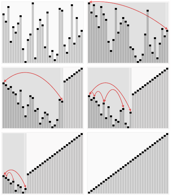
The Selection-sort algorithm divides the input vector into two parts: a sorted subvector of items which is built up from left to right at the front (left) of the vector and a subvector of the remaining unsorted items that occupy the rest of the vector.

Initially, the sorted subvector is empty and the unsorted subvector is the entire input vector. The algorithm proceeds by finding the smallest (or largest, depending on sorting order) element in the unsorted subvector, exchanging (swapping) it with the leftmost unsorted element (putting it in sorted order), and moving the subvector boundaries one element to the right.

Selection sort animation.
Red is current min.
Yellow is sorted list.
Blue is current item.

template <typename elem>

void sel_sort (vector<elem>& v) {
    int n = v.size();
    for (int i = 0; i < n - 1; ++i) {
        int p = pos_min(v, i, n-1);
        swap(v[i], v[p]);
    } 
}

template <typename elem>

int pos_min (vector<elem>& v, int l, int r) {
    int p = l;
    for (int j = l + 1; j <= r; ++j) {
        if (v[j] < v[p]) p = j; 
    }
    return p;
}

Insertion-sort

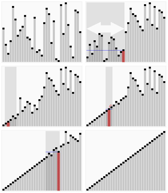
Insertion sort iterates, consuming one input element each repetition, and grows a sorted output list. At each iteration, insertion sort removes one element from the input data, finds the location it belongs within the sorted vector, and inserts it there. It repeats until no input elements remain.

Insertion sort animation

template <class T>

void insertion_sort (vector<T>& v) {
    int n = v.size();
    for (int i = 1; i < n; ++i) {
        for (int j = i; j > 0 and v[j - 1] > v[j]; --j) {
            swap(v[j - 1], v[j]);
        } 
    } 
}

Merge-Sort

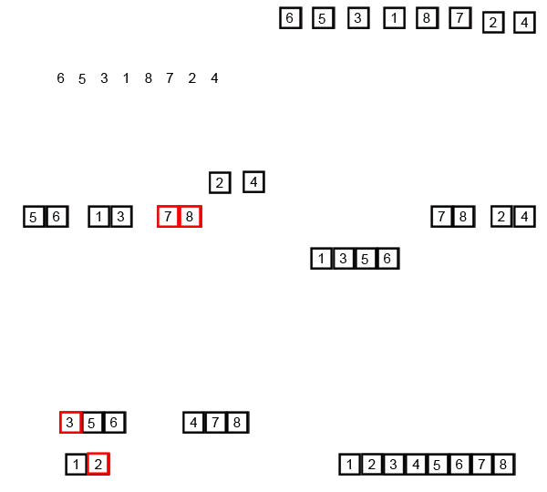
Merge sort is a divide-and-conquer algorithm that was invented by John von Neumann in 1945. Conceptually, a merge sort works as follows:

1. Divide the unsorted list into n sublists, each containing one element (a list of one element is considered sorted).
2. Repeatedly merge sublists to produce new sorted sublists until there is only one sublist remaining. This will be the sorted list.

An example of merge sort. First, divide the list into the smallest unit (1 element), then compare each element with the adjacent list to sort and merge the two adjacent lists. Finally, all the elements are sorted and merged.

template <class T>

void mergesort (vector<T>& v) {
    mergesort(v, 0, v.size() - 1);
}

void mergesort (vector<T>& v, int l, int r) {
    if (l < r) {
        int m = (l + r) / 2;
        mergesort(v, l, m);
        mergesort(v, m + 1, r);
        merge(v, l, m, r);
    } 
}

void merge (vector<T>& v, int l, int m, int r) {
    vector<T> b(r - l + 1);
    int i = l, j = m + 1, k = 0;
    while (i <= m and j <= r) {
        if (v[i] <= v[j]) b[k++] = v[i++];
        else b[k++] = v[j++];
    }
    while (i <= m) b[k++] = v[i++];
    while (j <= r) b[k++] = v[j++];
    for (k = 0; k <= r - l; ++k) v[l + k] = b[k];
}

Quick-Sort

Quicksort was developed by British computer scientist Tony Hoare in 1959 and published in 1961. It is still a commonly used algorithm for sorting. Overall, it is slightly faster than merge sort and heapsort for randomized data, particularly on larger distributions.

Quicksort is a type of divide-and-conquer algorithm for sorting an array, based on a partitioning routine; the details of this partitioning can vary somewhat, so that quicksort is really a family of closely related algorithms.

Applied to a range of at least two elements, partitioning produces a division into two consecutive non empty sub-ranges, in such a way that no element of the first sub-range is greater than any element of the second sub-range. After applying this partition, quicksort then recursively sorts the sub-ranges, possibly after excluding from them an element at the point of division that is at this point known to be already in its final location. Due to its recursive nature, quicksort (like the partition routine) has to be formulated so as to be callable for a range within a larger array, even if the ultimate goal is to sort a complete array.

The choice of partition routine (including the pivot selection) and other details can affect the algorithm’s performance, possibly to a great extent for specific input arrays.

Animated visualization of the quicksort algorithm. The horizontal lines are pivot values.

template <class T>

void partition(vector<T>& v, int l, int u, int& k) {
    int i = l+1;
    int j = u;
    T pv = v[i]; // simple choice for pivot
    while (i < j+1) {
        while (i < j+1 and v[i] <= pv) ++i;
        while (i < j+1 and pv <= v[j]) --j;
        if (i < j + 1) {
            swap(v[i], v[j]);
            ++i; 
            --j;
        }
    }
    swap(v[l], v[j]);
    k = j;
}

void quicksort(vector<T>& v, int l, int u) {
    if (u -l + 1 > M) {
        int k;
        partition(v, l, u, k);
        quicksort(v, l, k-1);
        quicksort(v, k+1, u);
    }
}

void quicksort(vector<T>& v) {
    quicksort(v, 0, v.size()-1);
    insertion_sort(v, 0, v.size()-1);
}

Heap-sort

Heap-sort was invented by J. W. J. Williams in 1964 and it can be thought of as

“an implementation of selection sort using the right data structure.”
(Skiena, Steven)

Like selection sort, heapsort divides its input into a sorted and an unsorted region, and it iteratively shrinks the unsorted region by extracting the largest element from it and inserting it into the sorted region. Unlike selection sort, heapsort does not waste time with a linear-time scan of the unsorted region; rather, heap sort maintains the unsorted region in a heap data structure to efficiently find the largest element in each step.

A run of heapsort sorting an array of randomly permuted values. In the first stage of the algorithm the array elements are reordered to satisfy the heap property. Before the actual sorting takes place, the heap tree structure is shown briefly for illustration.

#include <queue>

template <class T>

void heapsort (vector<T>& v) {
    int n = v.size();
    priority_queue<T> pq;
    for (int i = 0; i < n; ++i) {
        pq.push(v[i]);
    }
    for (int i = n-1; i >= 0; --i) {
        v[i] = pq.top();
        pq.pop();
    } 
}

The following table compares the running times in the worst, best and average case of the ordering algorithms above as functions of the number of elements n of the input vector.

Algorithm	Worst case	Best Case	Average case
Selection-sort	\Theta(n^2)	\Theta(n^2)	\Theta(n^2)
Insertion-sort	\Theta(n^2)	\Theta(n) (The best case input is a vector that is already sorted.)	\Theta(n^2)
Merge-sort	\Theta(n\log n)	\Theta(n\log n) Merge sort’s best case takes about half as many iterations as its worst case.	\Theta(n\log n)
Quick-sort	\Theta(n^2)	\Theta(n\log n) (simple partition)	\Theta(n\log n)
Heap-sort	\Theta(n\log n)	\Theta(n\log n) distinct keys	\Theta(n\log n)

Comparison-based sorting algorithm

A comparison-based sorting algorithm takes as input an array/vector [a_1,a_2,\dots ,a_n] of n items, and can only gain information about the items by comparing pairs of them. Each comparison is of the form \text{$a_i > a_j$?}

and returns YES or NO and counts a 1 time-step. The algorithm may also for free reorder items based on the results of comparisons made. In the end, the algorithm must output a permutation of the input in which all items are in sorted order (say increasingly).

For instance, Quicksort, Mergesort, and Insertion-sort are all comparison-based sorting algorithms. How efficient can be comparison-based sorting algorithms?

Theorem

Any deterministic comparison-based sorting algorithm must perform \Omega(n \log n) comparisons to sort n elements in the worst case.

More precisely, for any deterministic comparison-based sorting algorithm A, for all n \geq 2 there exists an input I of size n such that A makes at least \log_2(n!) = \Omega(n \log n) comparisons to sort I.

To prove this theorem, we cannot assume the sorting algorithm is going to necessarily choose a pivot as in Quicksort, or split the input as in Mergesort — we need to analyze any possible (comparison-based) algorithm that might exist.

Proof (sketch)

For a deterministic algorithm, the permutation it outputs is solely a function of the series of answers it receives (any two inputs producing the same series of answers will cause the same permutation to be output). So, if an algorithm always made at most k < \log_2(n!) comparisons, then there are at most 2^k < n! different permutations it can possibly output. But the total number of possible permutations is n!. So, there is some permutation it can’t output and the algorithm will fail on any input for which that permutation is the only correct answer.

The theorem above actually holds for randomized algorithms too, but the argument is a bit more subtle.